Certified Adversarial Robustness via Randomized Smoothing
Introduction
Adversarial attacks:
- In image networks, for a correctly classified input $x$ you can normally find $x' \in B(x, \delta)$ for small $\delta$ such that $x'$ is classified as something completely different
- i.e., adding indistinguishable noise can make something classified as a dolphin instead of a panda
- (This is an old paper so they were thinking in the context of vision networks)
Certifiable Robustness
- Prediction at point $x$ is verifiably constant in some neighborhood of $x$
- Tricky to use for large neural nets
Randomized smoothing:
- Method for turning any classifier into a smoothed classifier (in the $\ell_2$ norm)
- $\mathsf{Smoothed}_{\sigma}(f)(x)$ returns the mode of $f(X)$ for $X \sim N(x, \sigma^2 I)$
- Constant within a ball around $x$
- In the context of neural nets, done via monte carlo algorithms
Tight Bounds on Robustness Theorems
Theorem 1: Let $f:\mathbb{R}^d \to \mathcal{Y}$ be any function mapping to categories $\mathcal{Y}$, and let $\epsilon \sim \mathcal{N}(0, \sigma^2I)$. Let $g$ be the adversarially smoothed function with variance $\sigma^2$ (as defined above).
Then let $p_A$ be the probability of returning the most likely class $c_A$ and $p_B$ be the second most likely class. Define $\overline{p_B}$, $\underline{p_A}$ to be upper and lower bounds such that $\overline{p_B} \leq \underline{p_A}$.
Then
$$\mathsf{Smooth}(f)(x+\delta) = c_A$$for all $||\delta||_2 < R$ where
$$ R = \frac{\sigma}{2}(\Phi^{-1}(\underline{p_A}) - \Phi^{-1}(\overline{p_B})) $$Theorem 2:
Assume $\underline{p_A} + \overline{p_B} \leq 1$. Then for any $\delta$ with $||\delta||_2 > R$ there exists a base classifier $f$ consistent with the class probabilities for which $g(x+ \delta) \neq c_A$.
Monte Carlo Algorithms
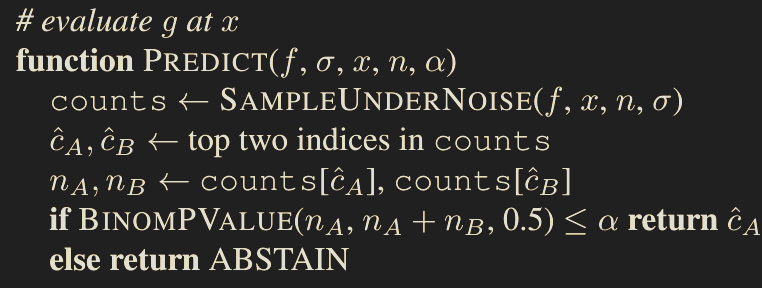
Hypothesis testing for the most points corresponding to the top class:
- Sample $N$ points
- Let $N_{[1]}, N_{[2]}, \ldots$ be the number of points in the most frequent, second most frequent, etc. class
- Idea: just look at $N_{[1]}$, $N_{[2]}$
- Look at number of points in $N_{[1]}$ conditioned on $N_{[1]}+N_{[2]}$. Should be distributed like $\text{Binom}(N_{[1]}+N_{[2]}, \frac{p_{[1]}}{p_{[1]}+p_{[2]}})$
- Let null hypothesis be $p_{[1]} = p_{[2]}$, so probability of getting that many points if the distribution is $\text{Binom}(N_{[1]}+N_{[2]}, \frac{1}{2})$
This means that if we want probability $\geq 1-\alpha$ of returning the most likely class, we can use this hypothesis test and abstain if the null is not rejected:
To determine the robustness radius, we also need lower / upper bounds $\underline{p_A}$ and $\overline{p_B}$.
One way to do this would be to:
- First learn the most likely class using $\mathsf{Predict}$
- Then take a $1-\alpha$ lower confidence interval to $\underline{p_A}$
- Then take $\overline{p_B} = 1-\underline{p_A}$
- Then return $\frac{\sigma}{2}(\Phi^{-1}(\underline{p_A}) - \Phi^{-1}(\overline{p_B}))= \sigma\Phi^{-1}(\underline{p_A})$ so long as $\underline{p_A} > \frac{1}{2}$

Large Sample Complexity for Large Radii
- Consider the case where the true radius is infinite, i.e., the base classifier always predicts the same thing
- Then the “certified” radius after drawing $n$ datapoints is $\sigma \Phi^{-1}(\alpha^{\frac{1}{n}})$
- This gives that for $R = k\sigma$, $$n = \frac{\log\left(\frac{1}{\alpha}\right)}{\log\left(\frac{1}{\Phi(k)}\right)} \approx \sqrt{2\pi}\cdot \log\left(\frac{1}{\alpha}\right)\cdot k\cdot\exp\left(\frac{k^2}{2}\right)$$ which grows extremely quickly in $k$
This means heuristically, it takes a long time to certify large radii.